In_class_2

Getting Started

Import packages

pacman::p_load(sf, tmap, sfdep,tidyverse, knitr,plotly)

Import attribute files and join

getwd() 

[1] "C:/kekekay/ISSS624/In-class_2"

hunan <- st_read("data/geospatial",layer = "Hunan") 

Reading layer `Hunan' from data source 
  `C:\kekekay\ISSS624\In-class_2\data\geospatial' using driver `ESRI Shapefile'
Simple feature collection with 88 features and 7 fields
Geometry type: POLYGON
Dimension:     XY
Bounding box:  xmin: 108.7831 ymin: 24.6342 xmax: 114.2544 ymax: 30.12812
Geodetic CRS:  WGS 84

hunan2012 <- read.csv("data/aspatial/Hunan_2012.csv") 

sfdep - time cube

hunan_GDPPC<- left_join(hunan,hunan2012)%>% select(1:4,7,15)

Joining with `by = join_by(County)`

1st - spatial layer

2nd - non spatial layer

Deriving contiguity weights: Queen’s method

wm_q <- hunan_GDPPC %>%   
  mutate(nb = st_contiguity(geometry),          
         wt = st_weights(nb, 
                         style = "W"),          
         .before = 1)

Global Spatial Autocorrelation

Computing local Moran’s I

use local_moran() of sfdep package to compute local moran’s I of GDPPC at county level

lisa <- wm_q %>% 
  mutate(local_moran = local_moran( 
    GDPPC, nb, wt, nsim = 99), 
    .before = 1) %>% 
  unnest(local_moran)

Time Series Cube

GDPPC <- read_csv("data/aspatial/Hunan_GDPPC.csv")

Rows: 1496 Columns: 3
── Column specification ────────────────────────────────────────────────────────
Delimiter: ","
chr (1): County
dbl (2): Year, GDPPC

ℹ Use `spec()` to retrieve the full column specification for this data.
ℹ Specify the column types or set `show_col_types = FALSE` to quiet this message.

GDPPC_st <- spacetime(GDPPC, hunan, 
                      .loc_col = "County",
                      .time_col = "Year")
is_spacetime_cube(GDPPC)

[1] FALSE

pacman::p_load(zoo,Kendall)

is_spacetime_cube(GDPPC_st)

[1] TRUE

GDPPC_nb <- GDPPC_st %>%
  activate("geometry") %>%
  mutate(nb =include_self(st_contiguity(geometry)),
         wt = st_inverse_distance(nb,geometry,
                                  scale = 1,
                                  alpha=1),
         .before = 1) %>%
  set_nbs("nb") %>%
  set_wts("wt")

! Polygon provided. Using point on surface.

Warning: There was 1 warning in `stopifnot()`.
ℹ In argument: `wt = st_inverse_distance(nb, geometry, scale = 1, alpha = 1)`.
Caused by warning in `st_point_on_surface.sfc()`:
! st_point_on_surface may not give correct results for longitude/latitude data

Computing GI*

gi_stars <- GDPPC_nb %>%
  group_by(Year) %>%
  mutate(gi_star = local_gstar_perm(
    GDPPC, nb, wt)) %>%
  tidyr::unnest(gi_star)

Performing Emerging hotspot analysis

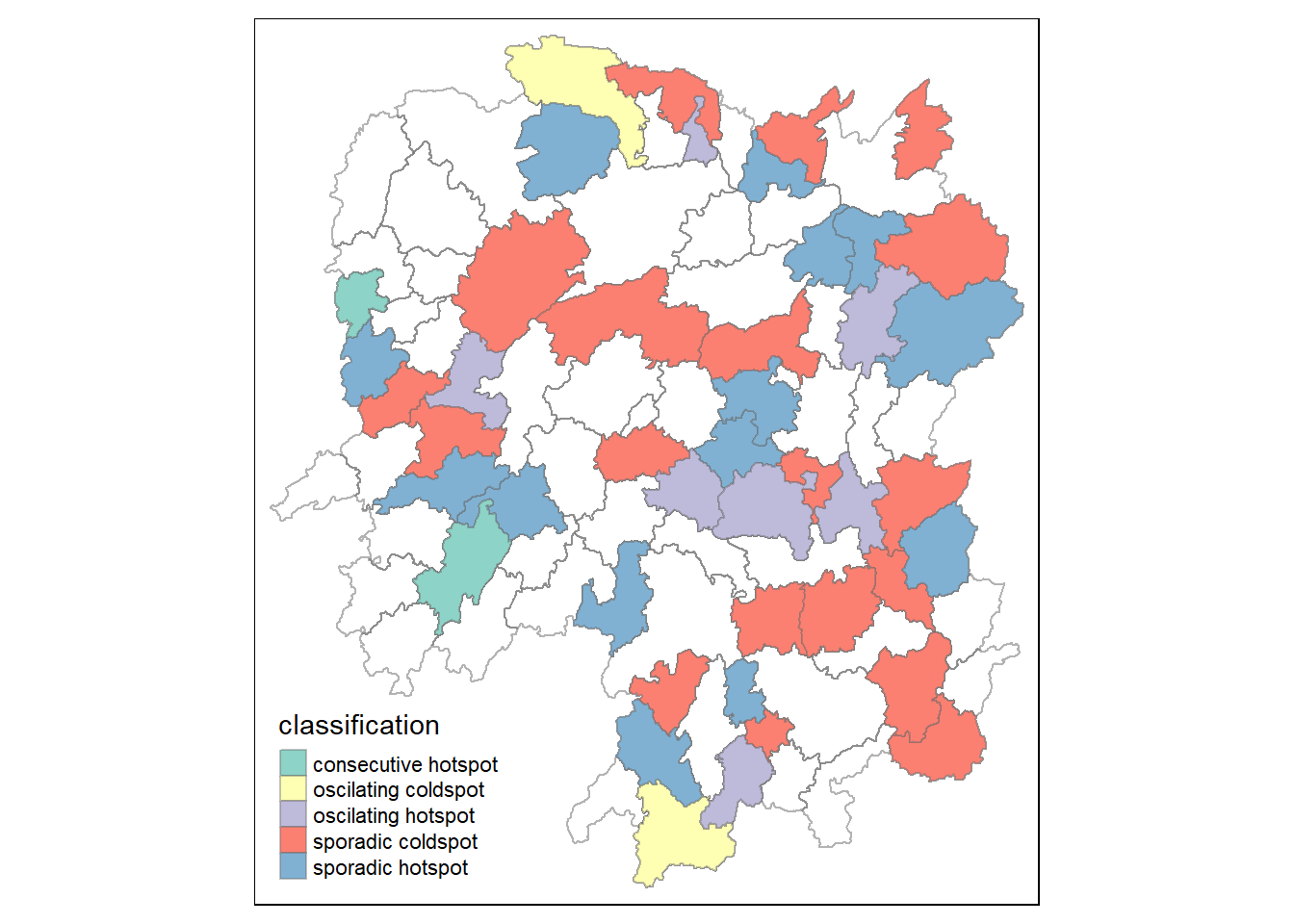
Visualising the distribution of EHSA classes

#install.packages("Kendall", repos = "https://cloud.r-project.org")
library(Kendall)

ehsa <- emerging_hotspot_analysis(
  x = GDPPC_st,
  .var = "GDPPC",
  k = 1,
  nsim = 99
)

hunan_ehsa <- hunan %>%
  left_join(ehsa,
            by = join_by(County==location))

ehsa_sig <- hunan_ehsa %>%
  filter(p_value < 0.05)

tmap_mode("plot")

tmap mode set to plotting

tm_shape(hunan_ehsa) +
  tm_polygons +
  tm_borders(alpha = 0.5) +
tm_shape(ehsa_sig) +
  tm_fill("classification") +
  tm_borders(alpha = 0.4)